Calculate Mean, Median and Mode in Excel – 3 Easy Formulas

Excel has some of really handy built in formulas that take away a lot of the manual work to calculate values. Included in these are formulas to quickly calculate Mean, Median and Mode. This simple guide will run through how to calculate each of the three.

Calculating Mean

Before we start with the formulas involved, let’s take a quick look at our sample dataset. Here we have 11 values representing various sales by two employees at a company:

Starting off with Mean. Calculating a mean in Excel can be done in two different ways. First is a standard calculation where we would individually sum each of the values and then divide the result by 11. A formula would look like:

=SUM(C3:C13)/11

This does the job, but Excel provides an even easier option in the form of the AVERAGE function. This formula essentially does the same thing as the above but counts automatically how many cells we are working with. In this case our formula would simply be:

=AVERAGE(C3:C13)

The output would then provide us with the average value of the sales below:

This calculation can go one step further by using a variation called AVERAGEIF. The syntax of this is as follows:

=AVERAGEIF(range, criteria, [average_range])

This essentially uses the rules of an IF formula by letting us apply a specific criteria to count the average on. In the above the range is going to be the employee name in column B, the criteria is the rule we are looking for, and average_range is the values. Let’s say we only want to see the average value of Steph’s sales – we could do this easily by using the below formula:

=AVERAGEIF(B3:B13,”Steph”,C3:C13)

Our result would be as follows:

Calculating Median

Moving on to Median. This simply counts the middle value based on all of the values after they have been sorted from lowest to highest. If we are working with an odd number of cases like we are in our set of 11 values then it will pick the middle value, however if there is an even number of cases we end up getting the average of the two middle numbers.

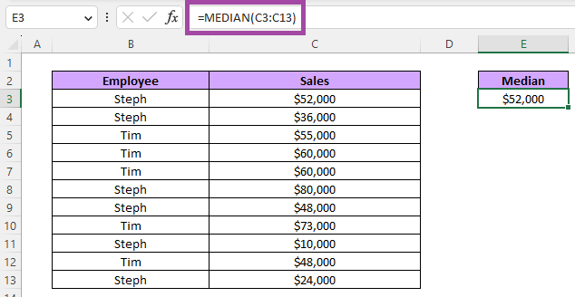
The formula for median is very straight forward here, with our formula looking like the below:

=MEDIAN(C3:C13)

This would then output the middle value of $52,000 as follows:

Unlike AVERAGE there is no MEDIANIF formula to work with here, although there is nothing stopping us from being creative and wrapping our formula with something like an IF and achieving a similar result.

Calculating Mode

Finally, let’s look at the formula for mode. This scans for the value that occurs the most in a dataset. There are two different versions of this formula that we can work with:

• MODE.SNGL – If there are multiple modes this only returns the first occuring set
• MODE.MULT – Returns an array of all modes. If there are multiple then it fills in more cells automatically

Using our same dataset, let’s look at the output for both of these options. The syntax for the two is identical other than the use of the SNGL or MULT phrase after MODE. Simply enter the range of values and we are good to go:

As we can see, MODE.SNGL presented an output of $60,000, while MODE.MULT displayed that same value but then also auto filled the cell below it with $48,000 – there is no formula entered into cell F4, only F3.

Since the pair of $60,000 happened before the $48,000 MODE.SNGL selected that as the mode to display.

Note that there is also the simple MODE formula but this is purely for compatibility with 2007 versions of Excel and earlier before these newer options were added.

Just like with MEDIAN there are no additional options such as MODEIF, but again with the right syntax there is nothing preventing us from going further into the formula with additional rules and filters.

This wraps up our guide on how to calculate Mean, Median and Mode in Excel. For more guides like this head over to our Excel category page.