How to easily merge data in Excel with a VLOOKUP

Working with multiple data sets in excel can be quite a time consuming and manual process. Depending on the complexity of the data and how much it needs cleaning there is often a fair bit to do in order to get it into a single clean sheet that you can work with for analysis or making visualizations.

This process becomes even more time consuming when working with multiple data sources where there needs to be some columns from one sheet merged into the master set. There are plenty of manual ways to go about this – which for smaller files is certainly do-able, although risky as it will likely involve copying and pasting figures which can easily lead to error.

This is where the VLOOKUP formula comes in handy!

Put simply, the VLOOKUP (short for Vertical Lookup) feature in Excel is a formula that works by taking a shared column that two or more separate data sets have, and using that as a ‘key’ in determining how to fill in a new column of data.

Lets look at an example.

Here we have two sets of data. The first containing the past months sales at a clothing store with each row listing out Sale ID, Product Name, Cost and Date of Sale. Each item also fits within a wider category that is only represented in the second table.

The VLOOKUP provides a really handy way of managing these classifications.

As you can see, the ‘Product’ column exists in both data sets. This will allow us to assign the Category column to the list of sales.

There is one big caveat here in order for the process to work. The ‘key’ column in the second data set needs to be unique values. If it appears over more than one row and contains a different value assigned to it then the formula will break as there is only one cell you are filling in a value for. There are alternative options for when we do have multiple values to return, but for a VLOOKUP in this case it needs to be unique. For example matching a capital city to it’s state – there is only one possible match.

Breaking down the formula

The structure for a VLOOKUP formula is as follows:

=VLOOKUP(lookup_value, table_array, col_index_num, [range_lookup])

This may seem a bit confusing, so let’s break the formula down piece by piece.

lookup_value: This one is quite straight forward – it is simply the location of the main value in the master data set that you are looking to use to search for when we scan the second data set. In this case you can either select the specific cell on that row (eg B2), or just the column as a whole (@B:B).

table_array: This part is the entire range of columns in data set two that you want to scan. The left most of these needs to be the key. You cannot have the shared values in column E and ask it to fill in your table with the values in column C for example. If this is the case you will need to manually cut and paste the columns in order. As you are looking to scan the entire column for the shared value you will need to set up the formula this way – for example E:F rather than E2:F2.

col_index_num: The purpose of this part of the formula is to tell Excel which column in the second dataset to fill in with. If your second data set has 5 columns overall (including the key), and the information you want to fill in with is in the 4th column, then enter ‘4’.

[range_lookup]: This one is optional, but highly recommended. There are two options for what you enter here – 1 or 0 (or TRUE or FALSE – they mean the same thing). 1 means that you will accept an approximate match, while 0 looks for the exact matching record. Approximate matching can be quite risky and inaccurate in most cases so would highly recommend using 0 by default.

Now that we have the formula broken out, lets go back to our example of categorizing store sales.

First we need to create a category column in the main table, and write the formula to scan the relevant cells. The first item we want to scan is in cell B2, with the columns we are referencing from the second table will be across H and I.

To start with, we need to enter the below formula into cell C2:

=VLOOKUP(B2,H:I,2,0)

This creates the initial reference point of that rows product name, then lets Excel know the extra data sits across columns H and I, and to fill in data with what is sitting in the second of these columns – in this case category. Now we simply drag down the formula and the rest will fill in! The final result will look like the below:

In this example both tables are sitting within the same sheet in Excel, but if that second set of data was on another tab, the formula would simply change to the below (which happens automatically if you are filling out the formula by clicking on the columns rather than typing each character).

=VLOOKUP(B2,Sheet2!H:I,2,0)

Handling VLOOKUP errors

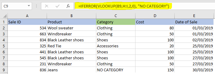
Going back to the [range_lookup] field, we may have cases where we choose an exact match but there is no shared value. This will typically result in an Excel error displayed as #N/A. As an extra workaround to this potential error, an IFERROR statement to wrap the whole formula will help! This simply adds an extra criteria for Excel to know that if the formula inside results in an error, fill the cell with the value we choose to enter instead. For example if we wanted a cell to say ‘NO MATCH’ if there is no match, then the formula would look like this:

=IFERROR(VLOOKUP(lookup_value, table_array, col_index_num, [range_lookup]),”NO MATCH”)

Things can get a bit complicated once we start wrapping formulas inside formulas, but this one is quite easy!

An example of this in action is below when working with the new product in cell B9 that was not in our lookup sheet:

This covers off the basic of working with VLOOKUPs. As we can see, they are a great way of filling in additional information such as creating classifications of data, or working with two separate data sets as long as the second data set has completely unique values in the shared column.

There are alternative methods to working with merging data, such as HLOOKUPS and INDEX and MATCH, but those will be covered off in separate articles.