How to Calculate Probability in Excel – Easy Formula

Probability is a measure that is calculated to determine the likelihood of something occuring. In this guide we will run through how to perform this analysis in Excel using a quick and easy formula.

Calculating Probability Using the PROB Formula

To calculate probability in Excel all we need to do is use the PROB formula. The syntax for this formula is as follows:

=PROB(x_range, prob_range, [lower_limit], [upper_limit])

Let’s break down each element of this:

• x_range: The range of values associated with the data we are measuring
• prob_range: A probability associated with each individual x value that is defined
• lower_limit: The lower limit on the range of values we want to measure probability of. Optional.
• upper_limit: The upper limit on the range of values we want to measure probability of. Optional.

The same dataset we are going to look at here is test scores and the probability of each occuring. Generally the figures we input here are based on historical results.

Our sample data from 0 – 100 looks like the below:

When working with data like this, in order for the probability calculations to work we need to ensure that the sum of all values in our second column adds up to 1 – or when converting to a percentage this means 100%. We can’t calculate the likelihood of various events if the sum of each doesnt total one hundred percent as that means we are missing a possible outcome.

Let’s say that based on the above we wanted to determine how likely it is that a student will score between 50 and 90. In this case the formula would need to cover cells B3 through B13 for the x range, C3 through 13 for the prob_range, and then we select B8 and B12 for our upper and lower limits. The formula would look like the below:

=PROB(B3:B13,C3:C13,B8,B12)

We are then presented with the following output:

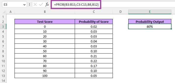
What this means is there is an 80% chance that when a student takes this test they will achieve a score of between 50 and 90.

This makes sense as if you were to manually sum up the values in column C from rows8 through to 12 they would total 0.80 which then converts to 80%.

Probability Without an Upper Limit

As mentioned above, the lower and upper limits in the PROB formula are optional. Let’s take a quick look at what would happen if we excluded the upper limit here as the results may not be quite what you are expecting.

Using the same lower range as our example we will only include cell B8 for our lower limit and leave it there. The returned output is then below:

This has resulted in a likelihood of just 10%. What this has done is only looked at the value against 50 which was 0.10. It could be easy to interpret removing the upper limit to mean something like ‘lower limit and above’ going all the way through to the highest possible value, rather than simply just look at the single lower limit.

If we did want to see lower limit and above we would need to be more explicit in specifying this by choosing cells B8 through to B13 for the 50-100 range.

With basic examples of calculating probability like this one it does feel slightly pointless to use the PROB formula here as we could simply just look at the 0.10 value in row 8 and that is our output value right there. Like all things in statistics however things can be far more complex so the lower limit only can be useful when paired with other concepts such as probability of something occuring X number of times.

This sums up our quick and easy guide on the basics of calculating probability in Excel using the handy PROB formula. For more Excel guides including plenty of other statistic related tutorials be sure to check out our Excel page here.