How to Alphabetize in Excel in 2 easy ways
In this guide, we will run through 2 easy methods on how to alphabetize in Excel. We will cover:
- Sorting using the sort function
- Sorting using a filter
- How to work with multiple columns and priorities
Let’s start with the first option.
Alphabetize in Excel using sort
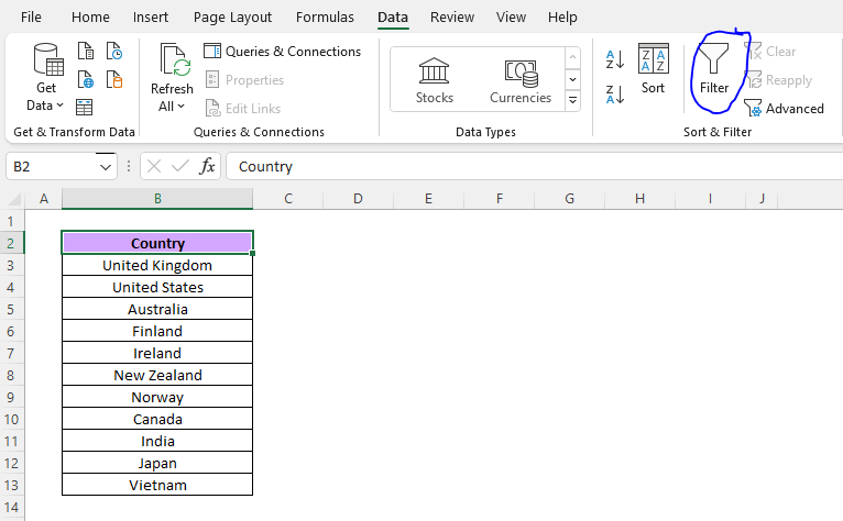
Let’s say we have a list of names in a single column, and we want to quickly and easily sort them in alphabetical order. In Excel this is super easy and only involves clicking a single button! First, we need to make sure we have selected one of the cells in the column, and then from there we go to the Data tab in the top ribbon, and simply click the little A-Z button!
This turns our list of countries form this:

To this:

Easy! Another nice plus is you will see there is a Z-A button as well, which as you may guess orders the names in reverse order.
You can also select the sort button itself, which pops up a box with more advanced options. If we leave everything as is and simply press OK then the result will be exactly the same as our first A-Z example. More on this pop up box later when we run through working with multiple columns.

Using a filter to Alphabetize
The next option works nicely is using Excel’s filter functionality. To activate this, select the column of data, and under the Data tab click on the filter button:
As we can see, a little drop down box has now appeared on the dataset. If we click into this the same A-Z and Z-A options appear. If we click these the exact same output as earlier occurs. The nice thing when working with filters is that it allows us to very quickly and easily apply things like alphabetizing without the need to go back into the data tab, or use that pop up box. We simply click on the columns filter button and choose the order.

Finally, let’s take a look at a more advanced option, where we have multiple columns that we want to alphabetize at once.
How to work with multiple columns
What if we have multiple columns that need to be not only put into alphabetical order, but we need to determine which is the higher level order of the two? This is where the Sort pop up box comes in again.
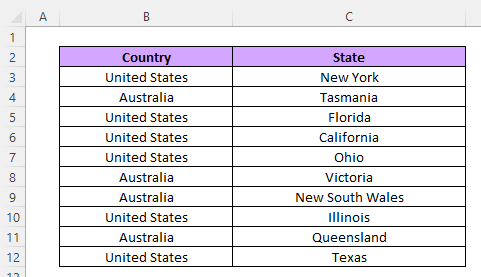
Using our example of countries, we have two countries in this case, the USA and Australia, and some states. Not only are we looking to sort the countries from A-Z, but we also want to make sure that within that the second column also then is sorted in alphabetical order as well as a second step.
Original data set:
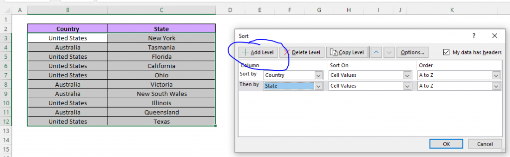
To start with, once we select the data and open up the sort box, make sure the country column is selected as A-Z, and from here press OK. As you can see from the output, the countries are now in order, but it has left the states in the exact same order they were within the context of the country column:
To fix this, jump back into the sort box, and click Add Level, and now select the State column and use the same A-Z sorting.
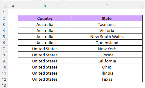
As you can see, we now have all of Australia, followed by all of the United States, but each of the states within the two are now also in alphabetical order:

This can make life really easy when we have a whole lot of columns that we want to work with and need to quickly create a hierarchy of sorting to be used in a report. This also works with numbers using a Smallest to Largest and vice versa rather than A-Z.
This sums up our guide on how to alphabetize in Excel. It is a very quick and easy function that makes cleaning and sorting our data quite painless.
For more handy guides on working with Excel, be sure to check out our Excel Tips page.