How to Print Gridlines in Excel in 3 Easy Ways
By default, when printing a workbook from Excel the gridlines that appear by default in the document itself will disappear in the printout itself. Sometimes this can make a document look cleaner, but often it makes things like tables a bit harder to actually read.
In this simple guide, we will cover how to print gridlines in Excel. We will cover:
- How to set gridlines to print from the page layout
- How to set gridlines to print from the print preview
- Alternative options
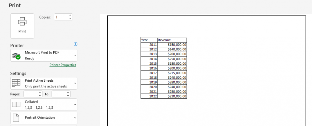
Before we move on to the two key approaches, let’s look at a quick set of data we have created with Excel, and how it would look by default when printed.
In Excel itself, with gridlines turned on, and no formatting applied our basic dataset of two columns looks like the below:

When heading up to print this page however the preview ends up looking like this:

Definitely cleaner, and with just the two columns it’s not necessarily hard to read, but if we had ten columns for example and working with a ton of data those lines can be helpful.
As mentioned, there are two key approaches for printing gridlines in Excel, and on top of that there is a third approach that is a bit different, and arguably the best approach. But first let’s start with one of the two standard approaches – the page layout options.
Print Gridlines in Excel using Page Layout
The first approach is pretty simple, and means that whenever we go to print this workbook the gridlines will appear.
First, under the ribbon head to Page Layout and the Gridlines section, simply tick the Print box:

Now when we head back to our print preview option we can see the gridlines surrounding our dataset:

Let’s now have a look at the other approach.
Using Print Page Setup for Gridlines
The second option to print gridlines in Excel is to use the page setup options within the print section itself.
After entering the print preview section, press the Page Setup button at the bottom, and then under the Sheet tab tick the Gridlines box:

This results in the exact same output as the first option.
Finally, let’s discuss an alternative option.
Using formatting to Print Gridlines
The third option to print gridlines in Excel is to use formatting to create the illusion of them being there. In a lot of cases this is actually probably the best approach as it let’s us make the document look a lot more professional and slick if we want it to – and in some ways is probably part of why the gridlines themselves are turned off for printing by default.
To achieve this, highlight every cell in our table, and in the font section of the Home Ribbon, click into the borders box and select whichever type of borders yo uwould like – in this case we have gone with All Borders just so every possible line can be filled in.

The table will now look like the below, with darker lines that are distinct from the gridlines themselves:

From here, when we go to print the output in print preview even with gridlines turned off will look like this:
As mentioned, this option is a great one as it really allows for a lot more formatting. We can give colour to the headers, thicker borders and so on to really make our printed output look a lot nicer.
This sums up our guide on how to Print Gridlines in Excel. For more handy guides on working with Excel, be sure to check out our Excel Tips page.